Introduction to Data Science - Using Python in the newsroom

Now that we're comfortable with our coding environment, and we've dabbled with the iPython notebook, it's time to dive into pandas, the Python library created explicitly for data analysis. This library, and this lesson, are intended to be used interactively, though they can also be saved in functions and scripts for later use.

Our iPython notebooks for this lesson are in our Github repo. You'll want to start with this one to follow along. Download the text, save it to an ipynb file in the same directory as the data and open it in iPython Notebook. You can also download it or view it here.

First in our interactive iPython notebook, we'll import pandas and call it "pd", a convention of pandas users that you'll quickly grow accustomed to.

import pandas as pd

Today, we're going to work with a fairly large text file of car accident data from the New Jersey Department of Transportation. This file contains reports from accidents in the Garden State between 2008 and 2013. The data, originally filed in handwritten reports by state troopers and then typed into a fixed-width database by clerks, is both decently large and very messy. (As an aside, if you're really interested in the genesis of this particular file, you can browse the makefile we used to create it.)

Our analysis today will not be comprehensive or particularly accurate, but working with 1.7 million rows of dirty data is a pretty good way to illustrate what you can do with pandas and how it's going to make your life easier.

The first thing we have to do is ingest our data from a source into a pandas DataFrame object. Think of a DataFrame (similar to R's Data Frame) as a virtual spreadsheet. It has columns with unique names and rows with unique row numbers, which we call "the Index". You can read in data from many kinds of sources: json, Excel files, html on the web, sql databases or others. Today, we're going to work with a CSV. First, we're going to create a variable with the name of our CSV, then we'll use pandas' .read_csv() function.

datafile = "njaccidents.csv"
df = pd.read_csv(datafile)

Now we have a DataFrame object with the name df. Does it look familliar?

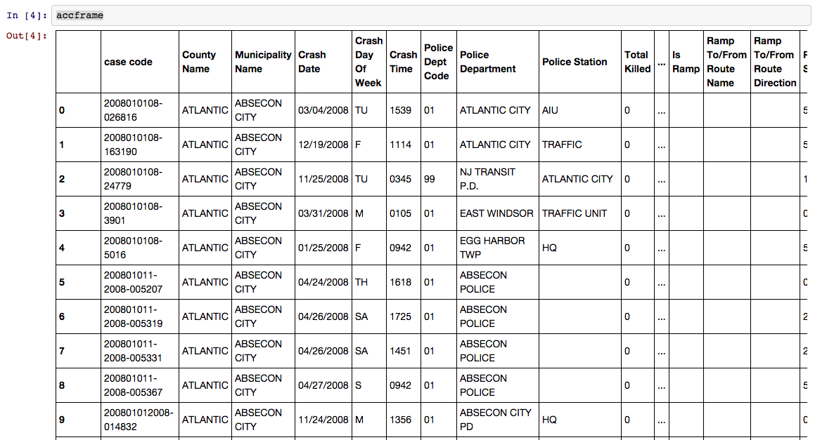
It's a table!

To see what we have here, let's make a list of the columns we have to work with the DataFrame's .columns attribute.

In [5]: df.columns
Out [5]: Index([u'case code', u'County Name', u'Municipality Name', u'Crash Date', u'Crash Day Of Week', u'Crash Time', u'Police Dept Code', u'Police Department', u'Police Station', u'Total Killed', u'Total Injured', u'Pedestrians Killed', u'Pedestrians Injured', u'Severity', u'Intersection', u'Alcohol Involved', u'HazMat Involved', u'Crash Type Code', u'Total Vehicles Involved', u'Crash Location', u'Location Direction', u'Route', u'Route Suffix', u'SRI (Std Rte Identifier)', u'MilePost', u'Road System', u'Road Character', u'Road Surface Type', u'Surface Condition', u'Light Condition', u'Environmental Condition', u'Road Divided By', u'Temporary Traffic Control Zone', u'Distance To Cross Street', u'Unit Of Measurement', u'Directn From Cross Street', u'Cross Street Name', u'Is Ramp', u'Ramp To/From Route Name', u'Ramp To/From Route Direction', u'Posted Speed', u'Posted Speed Cross Street', u'Latitude', u'Longitude', u'Cell Phone In Use Flag', u'Other Property Damage', u'Reporting Badge No.'], dtype='object')

To get a quick overview of what kind of data is in each column, we can try the describe method.

df.describe()

In earlier versions of pandas (<15), describe() gives you the summary statistics for the numeric columns. In newer versions of pandas, using the include='all' keyword will summarize all the columns.

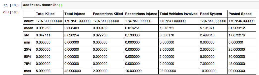
For categorical columns, you'll get the number of unique values and the most frequent. So this:

df['Severity'].describe()

returns this:

count     1707841
unique          3
top             P
freq      1326626
dtype: object

Say you want to select a single column. You can do this in one of two ways. If the column name is a string without spaces, you can use dot notation. like df.Severity, for instance. Otherwise, you use a similar syntax to what we're used to with dicts, using brackets like this: df['County Name']. If you want to grab more than one column, give it a list of column names. If you wanted to see the 'Cell Phone In Use Flag' column, or the 'County Name' column, how would you do it?

Now, let's take a look at cleaning messy data in columns. Why does this return an empty DataFrame?

df[df['County Name']=='PASSAIC']

With some digging, by using something like df[df['County Name'].str.contains('PASSAIC')], you'll notice that the 'County Name' column includes a bunch of trailing whitespace: 'PASSAIC '. Normally, in Python, you might solve this by writing a for loop to cycle through every item in the column and clean it up one at a time.

But with Pandas, we can do the same thing much faster. We'll use the regular Python .map() function to perform the .strip() method on every string in the column at the same time.

df['County Name']=df['County Name'].map(str.strip)

Now you go ahead and do the same for the 'Municipality Name' and 'Police Department' columns.

Once our 'County Name' field is cleaned, we can filter the table by its values, returning a view of the DataFrame that only shows rows with accidents that happened in Passaic County.

df[df['County Name']=='PASSAIC']

If we're confident the 'County Name' column is as clean as it's going to be, we can turn to others. What do we see when we look at the unique values in the 'Police Dept Code' column with the unique() method?

df['Police Dept Code'].unique()
array(['01', '99', '  ', '02', '03', '04', 1, 99, 2, 3, 4], dtype=object)

If we filter the column for the police departments that use '99' as their code, we'll see they're not unique (of course).

df[['Police Dept Code', 'Police Department']][df['Police Dept Code']==99]

You also might notice that some of our department codes start with 0, so we have data that is mixed between strings and integers in the same column. We can use pandas' .astype() method to change all the type of all of the values in that column to strings.

df['Police Dept Code']=df['Police Dept Code'].astype(str)

You should note two things here. To actually change the value of the column in the DataFrame in place, we'll have to assign it back to itself as if we're defining a new variable. Also, if you check the unique values again, we'll see that there are now values for '01' and '1'. You may want to standardize those, but we'll leave that to you as an exercise later.

Even after all that, we still have some empty fields with two spaces in the string, so let's replace those empty values with the word "Unknown"

df['Police Dept Code'][df['Police Dept Code']=='  ']='Unknown'

We've done a bit of cleaning here and may want to start doing some exploratory analysis. To do that, we'll create a smaller DataFrame of just the columns that we plan to examine, and we'll name it myframe.

myframe = df[['County Name', 'Municipality Name', 'Crash Date', 'Crash Day Of Week', 'Crash Time', 'Total Killed', 'Total Injured', 'Pedestrians Killed', 'Pedestrians Injured', 'Total Vehicles Involved', 'Crash Type Code', 'Alcohol Involved', 'Environmental Condition', 'Light Condition', 'Cell Phone In Use Flag']]

We'll pass myframe along to the next exercise for aggregating, but we might want to save it for later. While we're thinking about it, let's write it out to a CSV with the shockingly named to_csv() method.

myframe.to_csv('smallertab.csv')

Ready to dig deeper into pandas? Let's go.

Pandas, A First Look